Although every statistics book will tell you not to go looking for statistical significance, sadly that’s still what happens in many analyses and scientific research. Often forgotten, is to check for statistical power. Here’s a refresher, and how to do it in R.
Remember statistical significance?
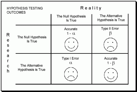
A finding is statistically significant if it is unlikely to occur when the null hypothesis is true.
Statistical power is its lesser known half-sister.
An alternative hypothesis has statistical power if you are unlikely to accept the null hypothesis when the alternative hypothesis is true.
I can make it more clear by referring to the confusion matrix. The probability of a Type I error is known as alpha (α). The probability of a Type II error is known as beta (β). The statistical power of a hypothesis is one minus beta (1 – β).

Here’s an example. You are comparing the weight of blue cars with red cars. Your hypothesis is that blue paint is more dense than red paint and that it adds a couple of grams to a car’s weight. You don’t have access to the paint.
So you start collecting blue and red cars. How many cars do you need to compare to confirm the alternative hypothesis if the weight difference is only a couple of grams? I’d say a lot. I would even dare to say that you’ll never find the necessary results to confirm your hypothesis, especially if you want to present some very significant results. This is exactly what we call statistical power of the alternative hypothesis. And in this case: it’s pretty dang low.
Statistical power of a t-test in R
To work with statistical power, we will use the pwr package. It has a very cool property because in its most important functions, you just need to drop one parameter and it will give you the value for that parameter, accounting for all the others.
In this first code snippet, I load the package, set the seed and generate two samples of data. I generate 25 blue and 25 red cards with an average of 1400 and 1400,05 kg and a standard deviation of 50(000) kilo(grams).
library(pwr)

set.seed(1988)

# Two samples, same standard deviation
standDev <- 50000
carCount <- 25

a <- rnorm(carCount,1400000,standDev) # red cars
b <- rnorm(carCount,1400050,standDev) # blue cars
If we do a t-test, we can clearly see that the the test does not pick up the difference, especially not on the p<0.05 level.
t.test(a,b)
So we can ask ourselves the question what the probability actually is for the test to pick up this difference. For this we can use the pwr.t.test function. We pass it the amount of element in each sample, the significance level we aim to achieve and Cohen’s D. This last parameter is a standardized measure of effect. In other words, it reports the effect size, but expressed in standard deviations. It’s a useful metric for comparing multiple studies on the same phenomenon.
cohensD <- (mean(a) - mean(b)) / standDev

test <- pwr.t.test(type='two.sample',
            n = carCount,
            sig.level = 0.05,
            d = cohensD)
test
In this example, the statistical power is only 0.08. This is extremely low, and we would like it to be as close to 1 as possible.

The statistical power depends on sample size. By plotting a pwr object, it will tell us the statistical power for a range of possible samples size. As you can see, the power increases along with the sample size. However, it appears we’ll never reach an acceptable level of statistical power.
plot(test)
But let’s say we change the mean difference of the samples to 25 kg or 25000 gram. What’s the statistical power in that scenario? As you can see, for a sample size of 25, it is between 0.5 and 0.75. By increasing the sample size to over 40, we could easily reach a level of 0.8.

Finally, you should keep in mind that statistical power is also a handy tool to determine sample size. If you have a prior hypothesis about the effect size of a phenomenon, and you have a desired level of confidence, you can use the concept of power to determine the necessary sample size.
By the way, if you’re having trouble understanding some of the code and concepts, I can highly recommend “An Introduction to Statistical Learning: with Applications in R”, which is the must-have data science bible. If you simply need an introduction into R, and less into the Data Science part, I can absolutely recommend this book by Richard Cotton. Hope it helps!
Great success!
Your point of view caught my eye and was very interesting. Thanks. I have a question for you. https://accounts.binance.com/zh-CN/register?ref=YY80CKRN